Tail-GAN: Comprehensive review and Implementation Insights
This project provides a comprehensive review and implementation insights of Tail-GAN, a generative adversarial network (GAN) architecture designed for modeling heavy-tailed distributions in financial data. The study delves into the architecture, training procedures, and performance evaluation of Tail-GAN, highlighting its effectiveness in capturing extreme events and tail dependencies in financial time series.
TL;DR
Tail-GAN is a GAN architecture tailored to match tail-risk measures like VaR and ES for trading strategies, using a specially designed score function. Here we review the theory and present an implementation based on an LSTM generator for stock prediction.
Introduction
The primary problem addressed in the paper is the accurate simulation and quantification of tail risk for benchmark trading strategies. Traditional Generative Adverserial Network (GAN)-based market generators, typically trained using cross-entropy or Wasserstein loss functions, may not adequately capture the tail properties of the distribution, which are critical for risk management applications. The reason being that tail risk measures may fail to be continuous for these divergence measures. Indeed, two probability distributions may have arbitrarily small cross-entropy of Wasserstein divergence yet widely different tail risk measures. This issue is addressed in the paper under analysis; “Tail-GAN: Learning to simulate tail risk scenarios” [1] by construction of a score function which quantifies closeness of the tails of two distributions with a theoretical guarantee of well-behaved optimization landscape.
The GAN
In the GAN framework, there is a discriminative model $D$, referred to as the discriminator, that learns the conditional probability of the target variable, given the input variable, or $P(Y|X=x)$. Examples of discriminative models are regression models. In addition to the discriminator, there is a generative model $G$, referred to as the generator, that learns the joint probability distribution of the input and output, or $P(X, Y) = P(X|Y)P(Y) = P(Y|X)P(X)$. The most common example of generative models is the naive Bayes model.
Now, let $P_d$ represent the distribution of our data $\textbf{x}$. In the standard GAN framework, a random sample $\textbf{z}$ from a noise distribution $P_z$ is first fed to the generator. The generator then outputs $G(\textbf{z})$, represented by the distribution $P_g$. A key aspect of $P_g$ is that its range is the domain of the real data distribution $P_d$. Those generated outputs, as well as the real data, are fed to the discriminator. The discriminator then attempts to make a distinction between the two, outputting a scalar representing the probability of its input belonging to $P_d$ rather than $P_z$. How close the discriminator was to predicting correctly is then back-propagated through both models. In each back-propogation, the discriminator aims to maximize the probability of assigning the correct label to both training examples and samples from the generator, while the generator updates $P_g$ with the aim of minimizing $\log(1 - D(G(z)))$.
This process is referred to as the adversarial process, where $D$ and $G$ play a two-player max-min game where $G$ plays the role of a counterfeiter who generates similar data as the real data, while $D$ plays the role of the judge to distinguish between the real data and generated data.
In the original paper ([2], proposition 2), Goodfellow et al prove that if $G$ and $D$ have enough training time and capacity, this max-min game terminates at a saddle point (a minimum with respect to one player’s strategy and a maximum with respect to the other player’s strategy) representing the state where the discriminator is unable to differentiate the two types of data. At this point, the generator has captured the data distributions, i.e. $P_g = P_d$. This saddle point is the optimum of the game’s value function $V(D,G)$, or
\[\min_{G}\max_{D}V(D,G) = \mathbb{E}_{\textbf{x}\sim P_d(\textbf{x})}\left[\log(D(\textbf{x}))\right] + \mathbb{E}_{\textbf{z}\sim P_z(\textbf{z})}\left[\log(1 - D(G(\textbf{z}))\right].\]In each learning step, we sample a mini-batch of $m$ examples from the noise distribution and the data distribution. We then update the discriminator by ascending its stochastic gradient:
\[\frac{\partial}{\partial \theta_d}\frac1{m}\sum_{i=1}^m\left[\log\left(D(x_i)\right) + \log\left(1 - D(G(z_i))\right)\right]\]and the generator by descending its stochastic gradient:
\[\frac{\partial}{\partial \theta_g}\frac1{m}\sum_{i=1}^m\log\left(1 - D(G(z_i))\right)\]where $\theta_d$ and $\theta_g$ are they weights of the discriminator and generator respectively, and $z_i,x_i$ are the $i-$th points of the noise sample and data respectively. One disadvantage worth mentioning is that that D must be synchronized well with $G$ during training in order to avoid “the Helvetica scenario” ($G$ collapses too many values of $\textbf{z}$ to the same value of $\textbf{x}$ to have enough diversity to model $P_d$)
Tail-GAN
Two commonly used statistics for measuring the tail risk of portfolios are the Value-at-Risk (VaR) and Expected Shortfall (ES). Given the gain $X: \Omega \to \mathbb{R}$ of the portfolio at a certain time $t$ and a probability measure $\mu$ on $\Omega$, the set of market scenarios, the VaR at confidence $0<\alpha<1$ is the $\alpha$-quantile of $X$ under $\mu$:
\[VaR_\alpha(\mu) := \inf \{x \in\mathbb{R}:\: \mu(X \leq x)\geq \alpha\}.\]ES is an alternative to VaR which is more sensitive to bigger tail losses and can be seen as the average loss that exceeds the VaR threshold:
\[ES_\alpha(\mu) = \frac{1}{\alpha} \int_0^\alpha VaR_\beta(\mu) \d \beta.\]Score functions for tail risk measures
We begin by giving the definition of elicitable functionals as explained in the paper by Lambert et al. [3]:
Definition 1: An elicitable functional is a statistical functional $T:\mathcal{F}\mapsto\mathbb{R}$ which admits a score function $S(x,y)$ such that
\[T(\mu) = \arg\min_x \int S(x,y) \mu(dy),\]for any $\mu \in \mathcal{F}$ where $\mathcal{F}$ is a set of distributions on $\mathbb{R}^d$.
It has been shown that $ES$ is not elicitable, whereas $VaR$ at level $\alpha \in (0,1)$ is elicitable for random variables with a unique $\alpha-$quantile. However, Fissler et al. [4], show that it is possible, under some conditions, to rewrite the tuple $VaR$ and $ES$ as a minimum as follows:
\[(VaR_\alpha(\mu), \: ES_\alpha(\mu)) = \arg \min_{(v,e) \in \mathbb{R}^2} \int S_\alpha(v,e,x) \mu(dx)\]The computation of the loss involves the optimization of the integral
\[s_\alpha(v,e) := \int S_\alpha(v,e,x)\mu(dx) = \mathbb{E}_\mu\left[S_\alpha(v, e, x)\right],\]and while there are infinite score functions $S$ that satisfy the necessary conditions, different choices lead to optimization problems, with some being easier than others. Proposed by Acerbi and Szekely [5], the following form of the score function has been adopted by practitioners for backtesting purposes:
\[S_\alpha(v,e,x) = \frac{W_\alpha}{2} (1_{\{x \leq v\}}-\alpha)(x^2-v^2) + 1_{\{x \leq v\}} e(v-x) + \alpha e \left(\frac{e}{2}-v\right), \quad \frac{ES_\alpha(\mu)}{VaR_\alpha(\mu)} \geq W_ \alpha \geq 1.\]Finally, the following proposition provides a guarantee for the well-behaved optimization landscape of the score function.
Proposition 1: Assume $VaR_\alpha(\mu) < 0$, for $\alpha < 1/2$. Then the score $s_\alpha(v,e)$ based on is strictly consistent for $(VaR_\alpha(\mu),ES_\alpha(\mu))$ and the Hessian of $s_\alpha(v,e)$ is positive semi-definite on the region
\[\mathcal{B} = \{(v, e) | v \leq VaR_\alpha(\mu), and W_\alpha v \leq e \leq v \leq 0\}.\]In addition, we assume there exist $\delta_\alpha \in (0, 1), \epsilon_\alpha \in(0, \frac1{2}-\alpha), z_\alpha\in(0, \frac1{2}-\alpha)$, and $W_\alpha > \frac1{\sqrt{\alpha}}$ such that
\[\frac{\mu(dx)}{dx}\geq \delta_\alpha \text{ for }x\in[VaR_\alpha(\mu), VaR_{\alpha+\epsilon_\alpha}(\mu)] \text{ and } ES_\alpha(\mu) \geq W_\alpha VaR_\alpha(\mu) + z_\alpha\]Then the Hessian of $s_\alpha(v,e)$ is positive semi-definite on the region
\[\tilde{\mathcal{B}} = \{(v, e) | v \leq VaR_{\alpha+\beta_\alpha}(\mu), \text{ and }W_\alpha v + z_\alpha \leq e \leq v\leq 0\} \text{ where }\beta_\alpha = \min\left\{\epsilon_\alpha, \frac{z_\alpha\delta_\alpha}{2W_\alpha}\right\}\]Proof is given in Appendix A of [1]
The minimizer of $s_\alpha(v,e)$ specifically $(VaR_\alpha(\mu),ES_\alpha(\mu))$, is located on the boundary of region $\mathcal{B}$ and $\tilde{\mathcal{B}}$ includes an open ball centered at $(VaR_\alpha(\mu),ES_\alpha(\mu))$. In essence, $s_\alpha(v,e)$ has a positive semi-definite Hessian near the minimum, ensuring favorable convergence properties. This provides a robust method for integrating tail risk measures into the GAN framework as an objective score function.
Model Setup
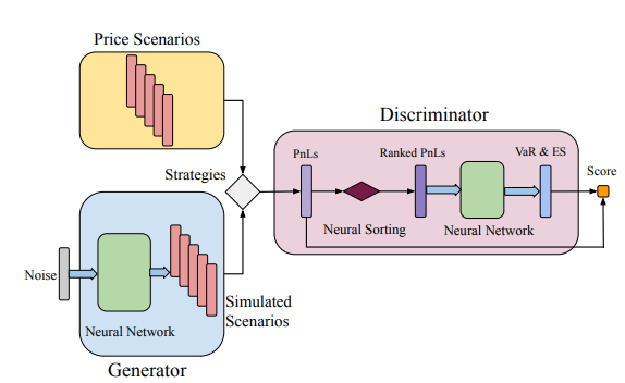
Let’s delve deeper into how the Tail-GAN is made and analyze each part. The generator simply generates samples that try to mimic the tail distribution of the training data. The discriminator tries to understand the quality of the generated samples using tail risk measures, across a set of benchmark strategies. To train the generator and the discriminator, we use a score function that uses the elicitability of VaR and ES as explained before.
Now, consider $M$ assets and $K$ different trading strategies of interest. Denote $\textbf{p} = {(p_{m,t})^T_{t=1}}^M_{m=1}$ as the matrix of the prices of each asset at the beginning of consecutive time intervals with duration $\Delta$. The same amount of capital is allocated to each strategy and they can operate at fixed time intervals. Furthermore, they need to be self-financing. Consider $K$ benchmark strategies to analyze the performance of the generator. For each strategy, a mapping $\Pi^k: \R^{M \times T} \to \R$ is defined to map the price scenarios $\textbf{p}$ to the final PnL at terminal time $T$.
Discriminator
With the aforementioned setup, the discriminator takes strategy PnL distributions as inputs and outputs two values for each of the $K$ strategies, aiming to provide the correct $(VaR_\alpha, ES_\alpha)$. Since the PnL distribution as well as the distribution of $\textbf{p}$ are impossible to access, we only show this as a sample-based approach. The more measure theoretic approach is also given in the original paper but will not be discussed here as the theory is of less focus as apposed to the model itself. To this end, we consider price samples ${\textbf{p}}_{i=1}^n$ with a fixed size of $n$ for the input of the discriminator. Recall that
\[(VaR_\alpha, ES_\alpha) = \arg\min_{(v,e)\in\mathbb{R}^2}\mathbb{E}\left[S_\alpha(v,e,x)\right]\]Mathematically, this amounts to
\[D^* \in \arg \min_D \frac{1}{K} \sum^K_{k=1} \frac{1}{n}\sum_{i=1}^n \left[S_\alpha(D(\Pi^k(\textbf{p}_j), j \in [n]);\textbf{p}_i)\right]\]where $\Pi^k(\textbf{p}_j), j \in [n]$ are PnL samples for strategy $k$ and $D(\Pi^k(\textbf{p}_j), j \in [n])$ is the VaR and ES prediction of $D$.
Given that the goal of the discriminator is to predict the $\alpha-VaR$ and $\alpha-ES$, including a sorting function $\Gamma$ in the architecture design could potentially improve the stability of the discriminator.
For the discriminator, a neural network with $L \in \mathbb{Z}^+$ layer is used. The functional form of the discriminator is
\[D(\textbf{x}; \gamma) = \textbf{W}_L \cdot \sigma (\textbf{W}_{L-1}...\sigma(\textbf{W}_1\Gamma( \textbf{x})+\textbf{b}_1)...+\textbf{b}_{L-1})+ \textbf{b}_L,\]in which $\gamma := (\textbf{W}, \textbf{b})$ represents the parameters in the neural network and $\sigma(\cdot)$ the activation function.
Generator
For the generator, a neural network with $J \in \mathbb{Z}^+$ layer is used. The functional form of the generator is
\[G(\textbf{z}; \gamma) = \textbf{W}_J \cdot \sigma (\textbf{W}_{J-1}...\sigma(\textbf{W}_1\textbf{z}+\textbf{b}_1)...+\textbf{b}_{J-1})+ \textbf{b}_J,\]A priori it is not known how big $G(\textbf{z}, \delta)$ has to be, but there exists a universal approximation under VaR and ES criteria(Theorem 3.3 [1]) which helps in taking this decision. The theorem implies that, under some reasonable assumption, a feed-forward neural network with fully connected layers of equal-width is capable of generating scenarios which reproduce the tail risk properties for the benchmark strategies with arbitrary accuracy. These assumptions are in regard to boundedness and continuity of $P_d, P_z$ and $\Pi$ which we will not cover here. To summarise, the use of this simple network architecture for Tail-GAN is justified. Additionally, the size of the network, namely the width and the length, depends on the tolerance $f$ the error $\epsilon$ and depends on $\beta$ in the case of ES.
As mentioned before, one of the disadvantages of the GAN framework is the need for synchronized training of $G$ and D. In this case, the loss function has to simultaneously account for the training of the generator and of the discriminator. This can be done by constructing a bi-level optimization problem and then applying the Lagrangian relaxation method with a dual parameter $\lambda>0$. By Theorem 3.6 [1], the following max-min game is equivalent to the bi-level optimization problem
\[\max_{D} \min_{G} \frac{1}{Kn} \sum_{k=1}^K \sum_{j=1}^n [S_\alpha(D(\Pi^k(\textbf{q}_i), \: i \in [n]), \: \Pi^k(\textbf{p}_j))-\lambda S_\alpha(D(\Pi^k(\textbf{p}_i), \: i \in [n]), \: \Pi^k(\textbf{p}_j))].\]where $\textbf{p}_i, \textbf{p}_j \sim P_d$ and $\textbf{q}_i \sim P_G, (i, j = 1, 2, . . . , n)$.
Again, this is the sample-based approach and the more measure theoretic approach is also given in the original paper.
The max-min structure encourages the exploration of the generator to simulate scenarios that are not exactly the same as what is observed in the input price scenarios, but are equivalent under the criterion of the score function, hence improving generalization.
The loss function of this architecture is more sensitive to tail risk and leads to an output which better approximates the $\alpha$-ES and $\alpha$-VaR values with respect to classical GAN loss functions.
Method
The following criteria was used to compare the scenarios simulated using Tail-GAN with other simulation models:
- Tail behavior comparison
- Structural characterizations
These evaluation criteria are applied throughout the numerical analysis for both synthetic and real financial data.
Tail Behavior Comparison
To evaluate how closely the VaR (ES) of strategy PnLs, computed under the generated scenarios, match the ground-truth VaR (ES) of the strategy PnLs computed under input scenarios, they employed both quantitative and qualitative assessment methods to gain a thorough understanding. For the quantitative assessment they constructed a performance measure to represent the overall measure of model performance, which they refer to as the average relative error of VaR and ES, by averaging over the relative error of VaR and ES, or
\[Re(n) = \frac1{2K}\sum_{k=1}^K\left(\frac{|VaR_\alpha(\Pi^k(\textbf{p}_i);i\in[n]) - VaR_\alpha(\Pi^k(\textbf{p}))|}{|VaR_\alpha(\Pi^k(\textbf{p}))|} + \frac{|ES_\alpha(\Pi^k(\textbf{q}_i);i\in[n]) - ES_\alpha(\Pi^k(\textbf{p}))|}{|ES_\alpha(\Pi^k(\textbf{p}))|} \right)\]where $n$ is the sample size. Additionally, they define the sampling error to be
\[Se(n) = \frac1{2K}\sum_{k=1}^K\left(\frac{|VaR_\alpha(\Pi^k(\textbf{p}_i);i\in[n]) - VaR_\alpha(\Pi^k(\textbf{p}))|}{|VaR_\alpha(\Pi^k(\textbf{p}))|} + \frac{|ES_\alpha(\Pi^k(\textbf{p}_i);i\in[n]) - ES_\alpha(\Pi^k(\textbf{p}))|}{|ES_\alpha(\Pi^k(\textbf{p}))|} \right)\]where again, $n$ the sample size but now the sample is from the data.
For the qualitative assessment they used rank-frequency distribution\footnote{A discrete form of the quantile function, i.e., the inverse cumulative distribution, giving the size of the element at a given rank} to visualize the tail behaviors of the simulated data versus the market data.
Structural characterization
To test whether Tail-GAN is capable of capturing structural properties, they calculated and compared the following statistics of the output price scenarios generated by each simulator:
- The sum of the absolute difference between the correlation coefficients of the input price scenario and those of generated price scenario
- The sum of the absolute difference between the auto-correlation coefficients (up to 10 lags) of the input price scenario and those of the generated price scenario.
Results
Information on the setup of parameters in the synthetic data set can be found in appendix B.1 in the original paper.
The authors tested the performance of Tail-GAN on a synthetic data set for which they could validate the performance of Tail-GAN by comparing to the true input price scenarios distribution. In this examination, 50,000 samples were used for training and 10,000 samples were used for performance evaluation.
Tail Behavior Comparison
Five financial instruments were simulated under a given correlation structure, with different temporal patterns and tail behaviors in the return distributions. The marginal distributions of these assets are:
- Gaussian distributions
- AR(1) with positive autocorrelation
- AR(1) with negative autocorrelation
- GARCH(1,1) with t-student noise
- GARCH(1,1) with a different t-student noise.
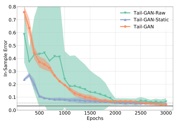
They examined the performance with one quantile value $\alpha = 0.05$. Figure shows the convergence of in-sample errors and Table below summarizes the out-of-sample errors.
| SE(1000) | Tail-GAN-Raw | Tail-GAN-Static | Tail-GAN | WGAN | |
|---|---|---|---|---|---|
| OOS Error (%) | 3.0 | 83.3 | 86.7 | 4.6 | 21.3 |
| (std. dev.) | (2.2) | (3.0) | (2.5) | (1.6) | (2.2) |
Table: Relative errors for out-of-sample tests. Mean and standard deviation (in parentheses).
Figure shows the in-sample errors of Tail-GAN, Tail-GAN-Raw and Tail-GAN-Static (WGAN is left out as it uses a different training metric). It can be seen that all simulations have a error convergence within 2000 epoch with errors smaller than 10% meaning that they all manage to capture the static information in the market data. Furthermore, table shows the Tail-GAN has the lowest training variance across multiple experiments meaning that it has the most stable performance. Moreover, the Tail-GAN far outperforms the WGAN which really depicts the success of the Tail-GAN. At last, Tail-GAN converges to an error $4.6\%$ while the other three models fail to capture the dynamic information in the data.
Structural characterization
Figures show the sum of the absolute difference between the correlation coefficients of the input price scenario(training data) and those of generated price scenario, and between the auto-correlation coefficients (up to 10 lags) of the input price scenarios and of generated price scenarios respectively. The numbers at the top of each plot denote the mean and standard deviation (in parentheses) of the sum of the absolute element-wise difference between the correlation matrices. Thus a lower number means better performance.
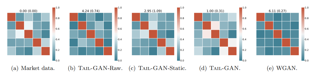
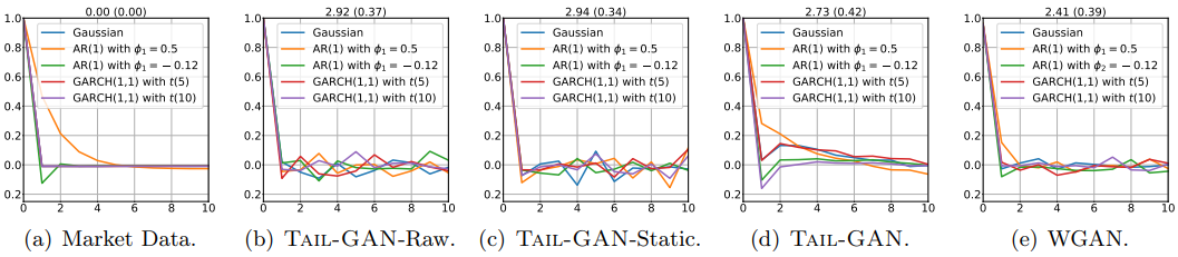
Figures demonstrate that the cross-correlations of the price scenarios are best reproduced by Tail-GAN. However, the auto-correlations are similar between models.
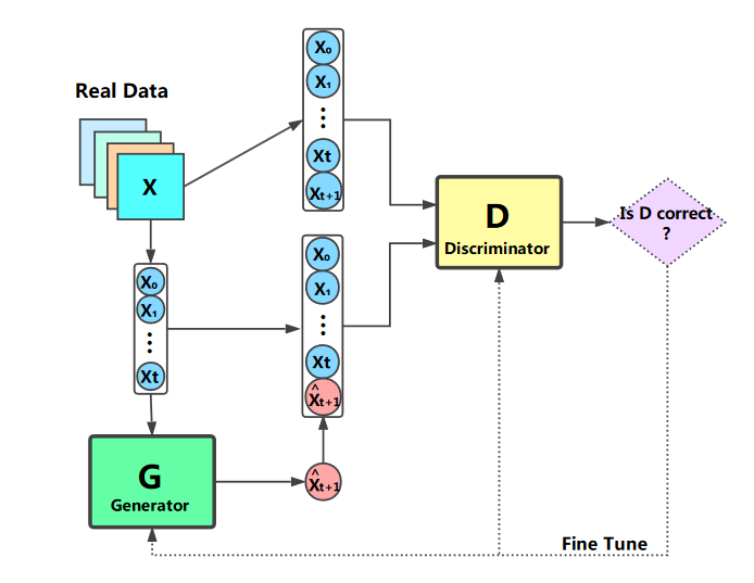
Implementation
After seeing how the Tail-GAN works we decided to implement a version of the GAN architecture by ourselves. We based the model on the framework presented in “Stock Market Prediction Based on Generative Adversarial Network” by Kang Zhang et al.[6]. We selected this framework due to the high computational power required by the original GAN, this meant excluding the portfolio valuation, PnL and (VaR, ES) computation. The resulting model provides a more accessible starting environment for applying GANs to financial time series prediction in hope of having more power to produce competitive results.
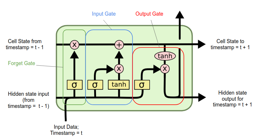
The authors of the Tail-GAN suggested that their model used the most basic architecture for the generator and that better and more complex models could be introduced. After some research on what was the best model to analyze time series data, we found out that the Long Short-Term Memory (LSTM) networks have the best performances. LSTMs, introduced by Hochreiter & Schidhuber [7], are a type of Recurrent Neural Network (RNN) that can learn long-term dependencies. They are particularly effective in overcoming the “vanishing gradient problem” of RNNs, where gradients used during training become extremely small, hindering the model’s ability to learn from long-term information. LSTMs consist of cells with 3 three main components called gates: the forget gate, the input gate, and the output gate. These gates regulate the flow of information through the cell:
- Forget gate: Decides what information from previous cell state should be thrown away or kept.
- Input gate: Determines which new information should be added to the cell state.
- Output gate: Decides what the next hidden state should be.
In an LSTM cell, information flows through three main components: the input, the hidden state (short term memory), and the cell state (long term memory). The input is the current data point, while the hidden state and cell state come from the previous time step. The current input and previous hidden state are combined and processed to update the cell state. The updated cell state and the processed information are then used to produce the next hidden state. This mechanism allows the LSTM to retain and update long-term information across sequences.
The discriminator was chosen to be a fully connected neural network just as it was presented in the Tail-GAN, just with a smaller number of neurons.
The generator loss function was inspired by the above-mentioned paper and it is the weighted sum of two components: the generator MSE loss and the cross-entropy one. This resulted in the following loss function:
\[G_{loss} = \lambda_1 \frac{1}{m} \sum_{i=1}^m (\hat{x}^i_{t+1} - x_{t+1})^2 + \lambda_2 \frac{1}{m} \sum_{i=1}^m \log(1-D(X_{fake})\]where $\hat{x}_{t+1}$ are the predictions made by the generator. Note that $\lambda_1, \lambda_2$ are manually set hyper-parameters (In our case 0.1 and 0.9 respectively).
Then the loss function for the discriminator is the typical binary cross-entropy function which was introduced before:
\[D_{loss} = -\frac{1}{m} \sum_{i=1}^m \log D(X_{real}) - \frac{1}{m} \sum_{i=1}^m \log (1-D(X_{fake}))\]where $D$ outputs binary values (0 or 1). The discriminator aims to output 0 for fake data and 1 for real data.
The stock data included six features: High Price, Low Price, Open Price, Volume and 5 days moving average and the objective is to predict the Adjusted Close Price. It can be seen that the first part is the one accounting for the Mean Square Error and the second one is the adversarial part.
We trained our model on real stock data, including highly volatile stocks like AAPL (Apple) and less volatile stock like KO (Coca Cola) with data sourced from Yahoo Finance. This choice was done based on the fact we thought that there would have been evidence of different prediction behavior (this was proven to be wrong). Training data excludes weekends and holidays to mimic real training conditions.
Normalization of the data is crucial for achieving competitive results, as emphasized in the original paper [6]. We normalize the data as follows:
where $\mu^t$ and $\tau^t$ are the mean and standard deviation of $\textbf{X}$. We empirically choose $t=5$ to predict the data on the next day using the past week’s data. The first 90% of the data is used for training, and the remaining 10% is used for testing.
Since the data was limited the problem of overfitting had to be tackled, after some research we found out that the dropout regularization [8] is needed. Dropout is a regularization technique in which some proportion of the neurons in a network are randomly “dropped out” or ignored during training, each with a given probability $p$. Furthermore as literature suggests [9] to have a better convergence and stability of the model it is recommended to perform Batch Normalization during the LSTM.
Our model focuses on the GAN framework to achieve almost-accurate stock price predictions, without accounting for extreme price jumps. Initial attempts using a fully connected neural network for the generator resulted in excessive computational time due to the high number of parameters (126 vs 1.7 thousands). Indeed the scope of our GAN is trying to mimic the price in every aspect while the Tail-GAN is just trying to match the tails. This bears the consequence that the Tail-GAN has a wider application use in the context of risk evaluation and risk management.
This configuration leverages the strength of LSTMs in handling time series data while simplifying the implementation for practical use in stock price prediction.
Experiments results
In order to assess the goodness of the GAN we decided to focus on different metrics such as RMSE, MAE and obviously the Generator and Discriminator loss. The result was the following plot:
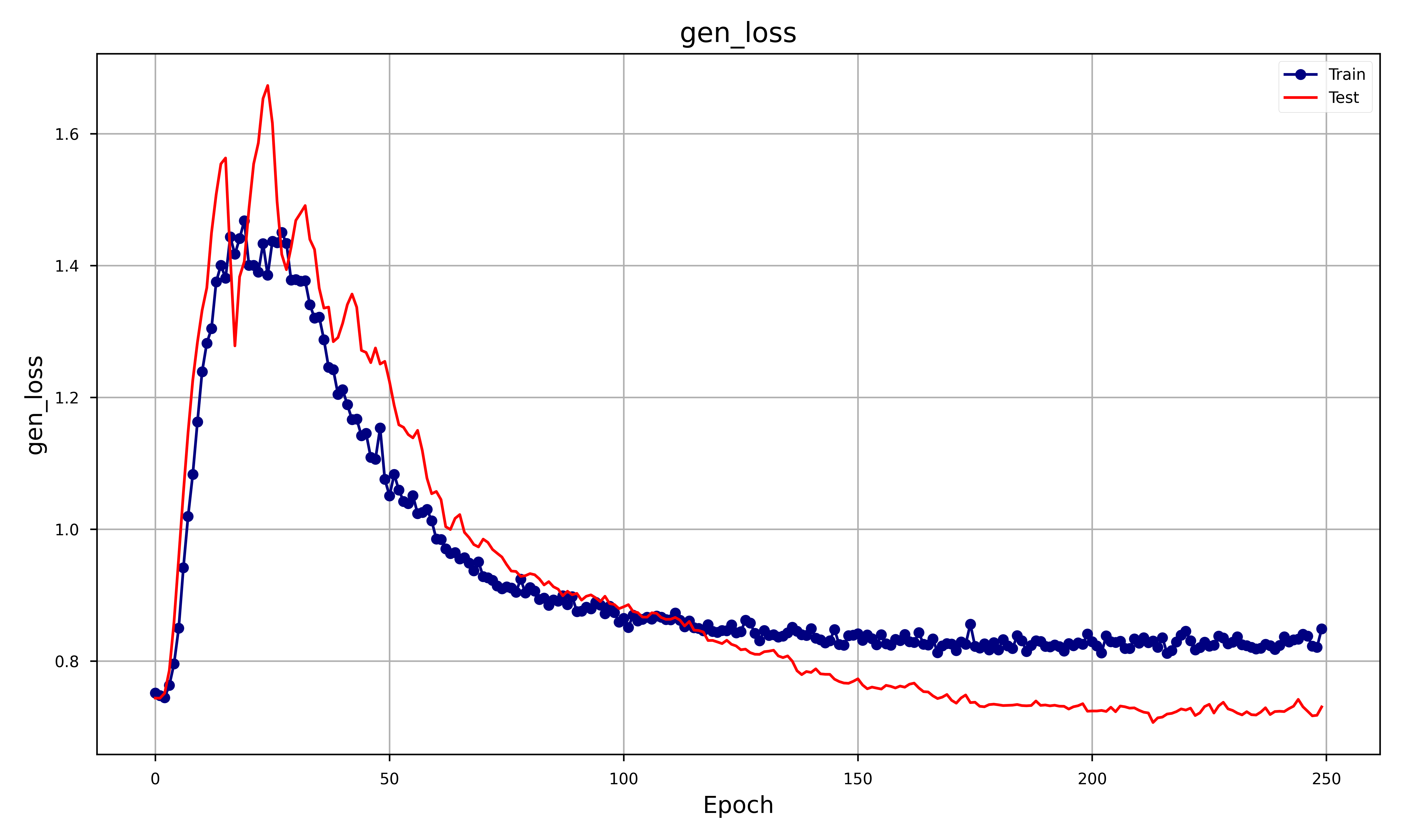
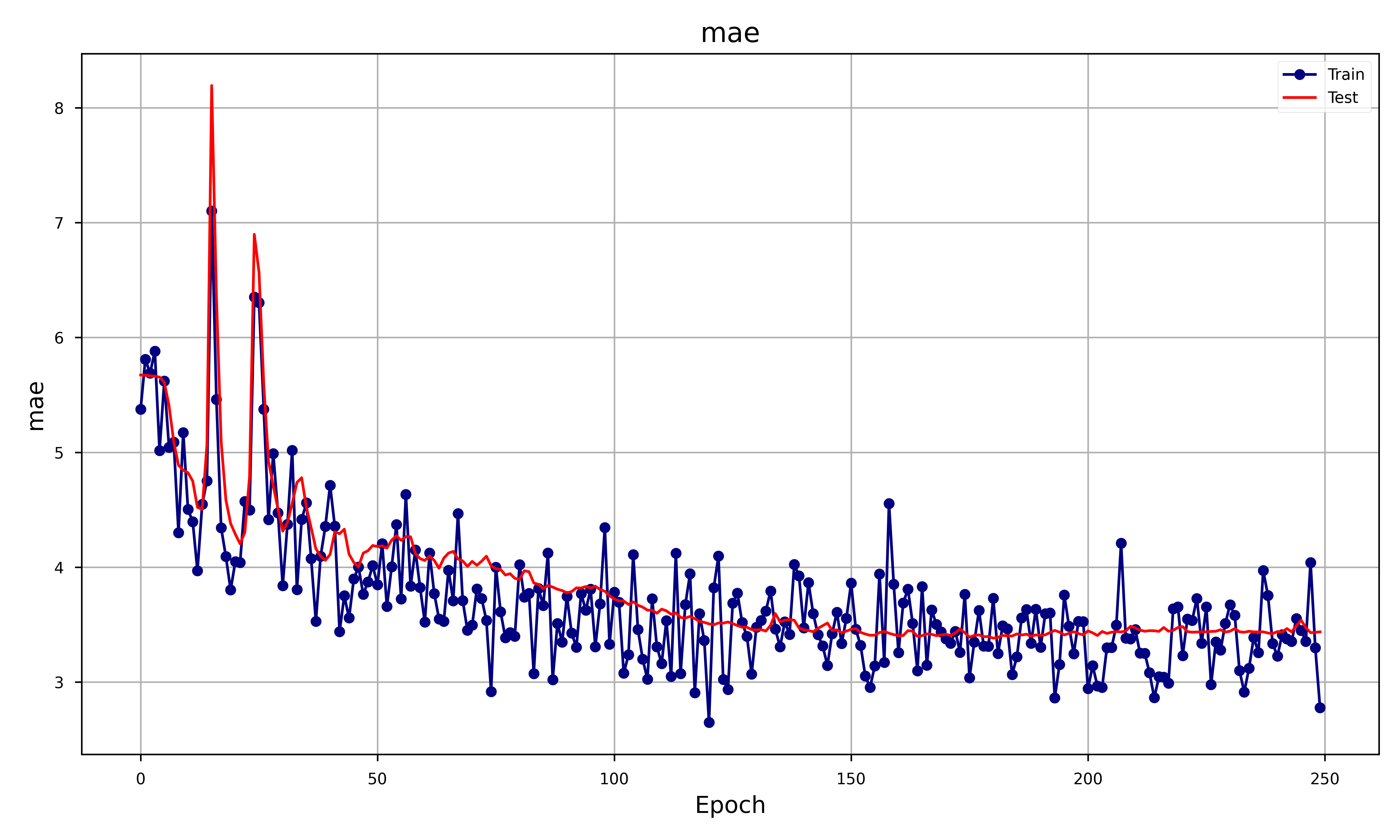
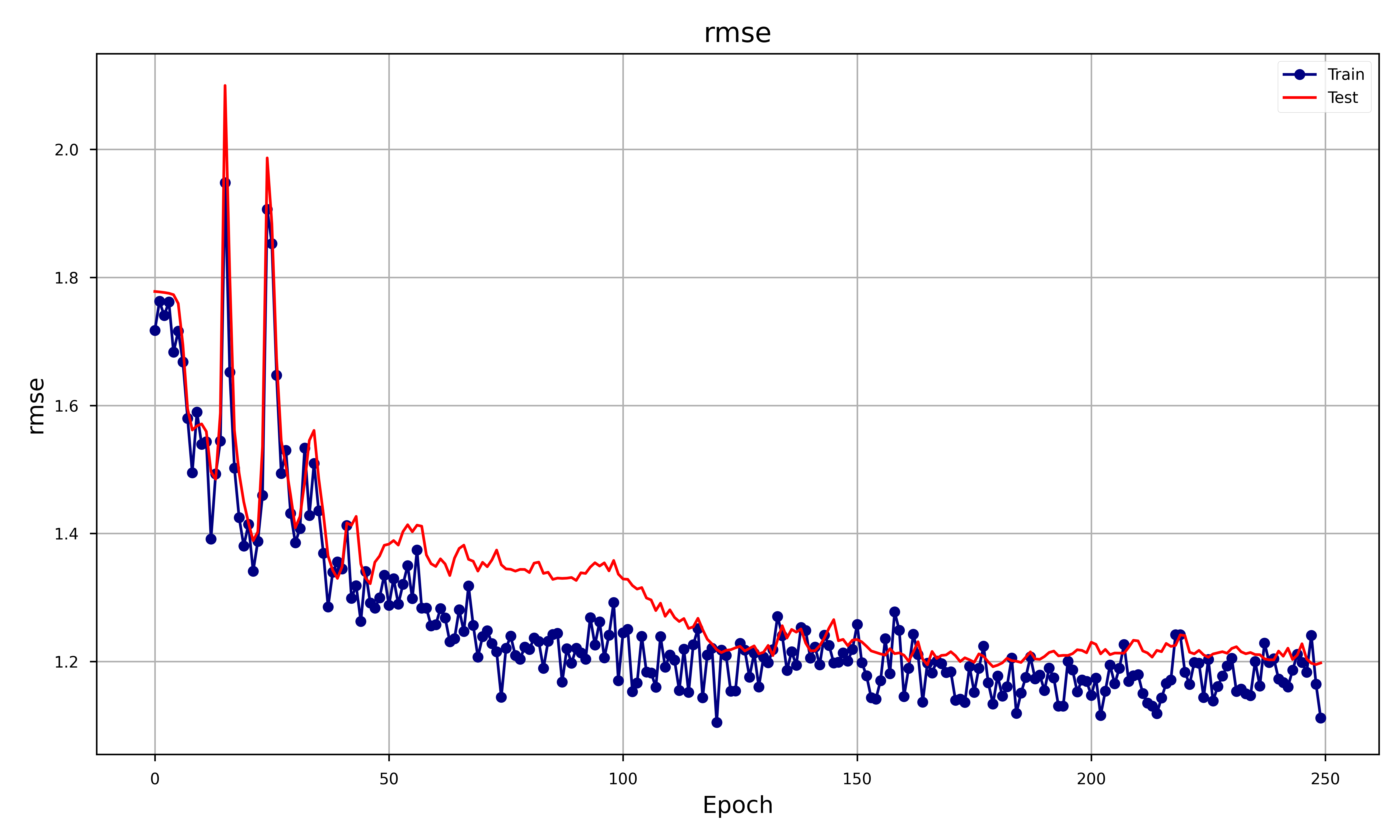
Let’s analyze each metrics and see how that behaves:
- Generator Loss: Both training and test generator losses start high and then decrease, but the training loss continues to decrease more steadily than the test loss. The training loss stabilizes after about 100 epoch.
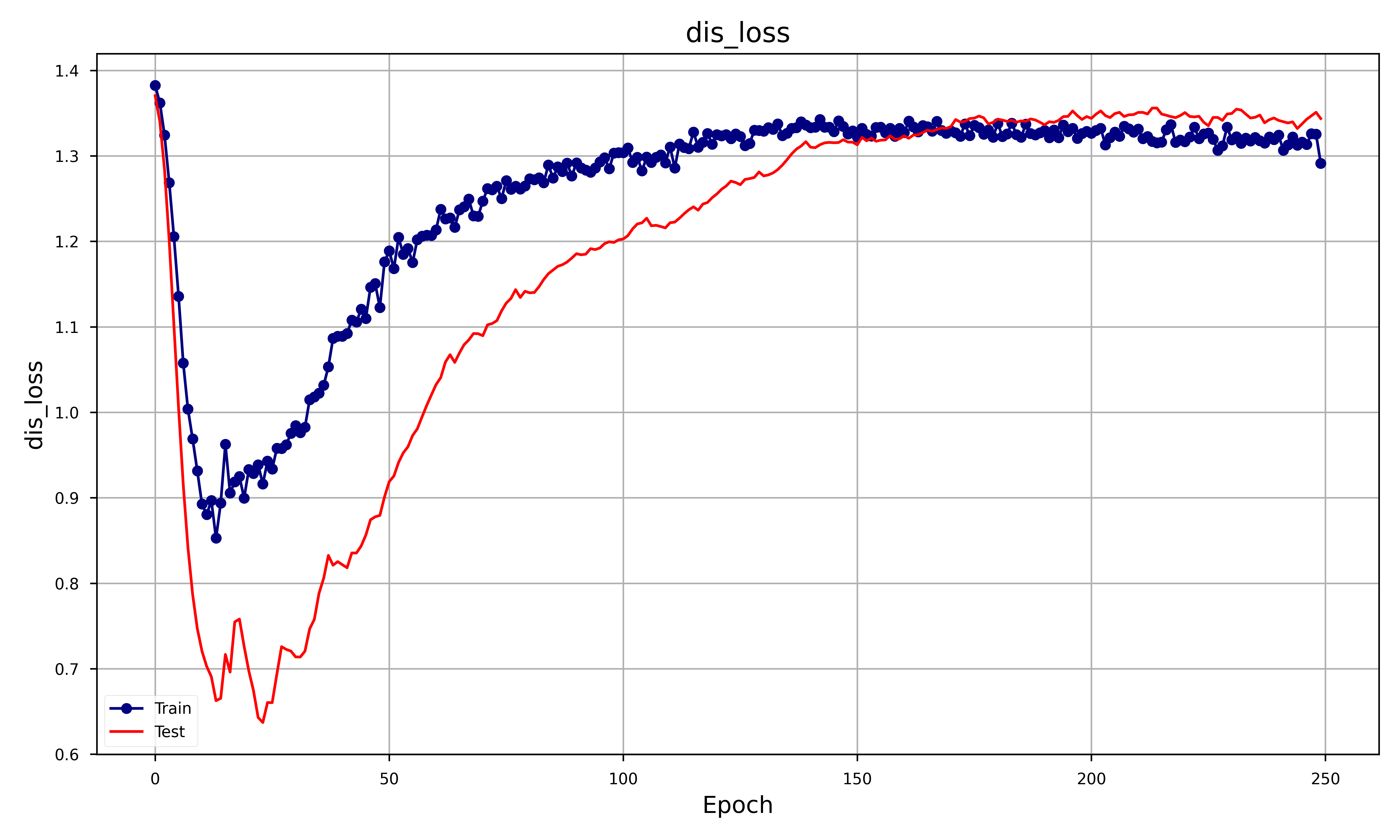
- Discriminator Loss: both losses start high, decrease sharply, and then start to increase again. The training loss consistently remains lower than the test loss. Both losses seem to stabilize after 150 epochs. The shape of the discriminator loss is exactly the one of the generator but flipped upside-down. This makes sense, since whenever the generator gets better at predicting (hence its loss decreases) the discriminator has a harder time triying to decide which price is the true one, hence its accuracy decreases (hence its loss increases).
- MAE: Both training and test MAE show a decreasing trend with similar behavior, stabilizing after around 100 epochs. This indicates that the generator is improving in generating realistic samples over time, but the close behavior of train and test curves suggests minimal overfitting.
- RMSE: The RMSE shows a similar trend to MAE with both training and test losses decreasing and stabilizing over time. Similar to MAE, the RMSE suggests that the generator’s outputs are becoming more accurate, with little overfitting.
Graphically, it can be seen that the GAN accurately depicts the overall shape of the price but, as expected, has some problems depicting when the stock has a big spike. This behavior is expected as the loss doesn’t inherently involve the analysis of extreme case scenarios, that is why the original paper was introduced.
Portfolio Testing
One application of our GAN could be the one of setting up portfolio strategies to maximize the returns. We set up an experiment in which we bought the stock at day one and kept it until it reached the highest peak in the price and then sold it to the real price (not the predicted one). We then benchmarked it with the theoretical return (the one obtained by the predicted price) and plotted it having the predicted outcome on the x axis and the real return on the y axis.
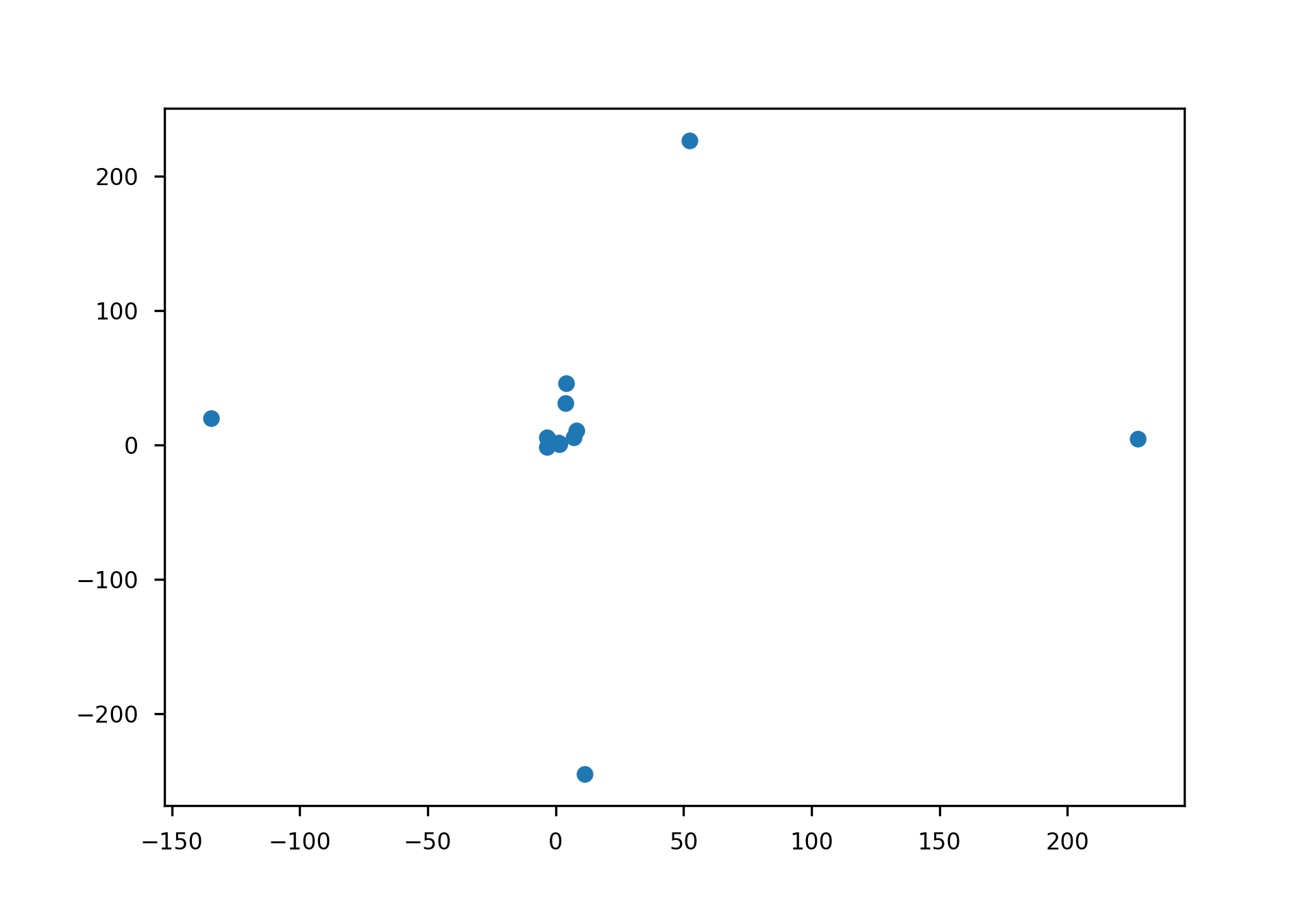
The mean of the predicted return is 7.62% and while the real return is 11.73%. While these results seem promising we have to keep in mind that in the plots the 75% outliers were removed. Indeed the worst scenario was the one in which the predicted return was 1.34% and the real one was -7000%. This is a result of the fact that the tail distributions aren’t matched and hence it was expected.
Conclusion and Discussion
The Tail-GAN aimed to address the significant challenge of simulation Tail-risk scenarios in financial markets. Traditional risk models often fail to capture extreme, rare events that can lead to catastrophic losses.
Throughout the report, the GAN model and evaluated its performance using synthetic data and real market scenarios. The results demonstrated that the architecture effectively generates realistic samples. Key metrics such as RMSE and MAE indicated minimal overfitting, and the model successfully captured the overall shape of stock prices, though it struggled with depicting some extreme spikes accurately.
In conclusion, the Tail-GAN project has made significant strides in improving the simulation of tail-risk scenarios. By advancing the capability to model extreme market events, Tail-GAN provides a valuable tool for financial institutions aiming to enhance their risk management strategies. However, continued research and development are necessary to fully realize its potential and address the remaining challenges in this complex field.
References
- R. Cont, M. Cucuringu, R. Xu, and C. Zhang, “Tail-GAN: Learning to Simulate Tail Risk Scenarios.” 2023.
- I. J. Goodfellow et al., “Generative Adversarial Net,” Proceedings of the International Conference on Neural Information Processing Systems, pp. 2672–2680., 2014.
- N. S. Lambert, D. M. Pennock, and Y. Shoham, “Eliciting properties of probability distributions,” Proceedings of the 9th ACM Conference on Electronic Commerce, 2008.
- T. Fissler and J. F. Ziegel, “Higher order elicitability and Osband’s principle,” The Annals of Statistics, vol. 44, no. 4, pp. 1680–1707, 2016, doi: 10.1214/16-AOS1439.
- C. Acerbi and B. Szekely, “Back-testing expected shortfall,” Risk, 2014.
- K. Z. et al, “Stock Market Prediction Based on Generative Adversarial Network,” IIKI 2018, 2018.
- J. S. Sepp Hochreiter, “Long short-term memory,” Neural computation, 1997.
- W. Zaremba, I. Sutskever, and O. Vinyals, “Recurrent neural network regularization,” arXiv preprint arXiv:1409.2329, 2014.
- T. Cooijmans, N. Ballas, C. Laurent, Ç. Gülçehre, and A. Courville, “Recurrent Batch Normalization,” arXiv preprint arXiv:1603.09025, 2016.